Modelling the kinetics of protometabolism
MSci Investigative Project | Lane Origins Group | UCL
How does one investigate the origin of metabolism? Although the origin of life and metabolism may seem obscure and unknowable, there is enough research and rigorous methods exist to test hypotheses about it. For my MSci Investigative Project in the Biological Sciences, I used advanced stochastic modelling techniques to investigate the kinetic requirements that would enable a primordial metabolic network to exist and propagate.
Background
Before we dive into mathematical models and mass-action kinetics, let's consider the theoretical background which underpinned my project: non-enzymatic protometabolism. There is biochemical and phylogenetic evidence to suggest that LUCA, the last universal common ancestor, was basal to Archaea and Bacteria. "Using “life as a guide” to its own origins" is a simple yet fascinating paradigm for investigating the origin of life. Accordingly, the core of modern metabolism is believed to be largely conserved between Archaea and Bacteria. As many will know, enzymes kinetically “speed up” already geochemically spontaneous reactions. However, under non-enzymatic protometabolism, the core of metabolism is thought to be
- Is parsimonious
- Bridges the gap between protometabolism and modern metabolism
- Resolves the end-product problem
For a more thorough map of protometabolism with this view, you can turn to Harrison S & Lane N. Life as a guide to prebiotic nucleotide synthesis. Nat Commun 9, 5176 (2018). Briefly however, in contrast to most experimental work to date, the Lane Origins group examines how metabolism arose from H2 and CO2 fixation, common to practically all living organisms:
- Sequential reactions of H2 with CO2 in biology gives rise to acetyl CoA and Krebs cycle intermediates
- Amino acids, fatty acids and sugars all derive from Krebs cycle intermediates
- Nucleotides derive from precursors shown in red boxes
As there are vastly different experimental conditions, modelling could help shrink experimental possibilities. Moreover, it opens the possibility to consider so many interesting questions:
- How much of modern metabolism can we recover, starting from CO2 and H2?
- How does the flux of matter propagate through the network?
- What are the bottlenecks?
- How robust is the network to changes in conditions?
- How (self)contradictory is the network?
Stochastic kinetic modelling: the Gillespie algorithm
Broadly, mathematical models can be thought of as existing on two spectra: from deterministic to stochastic; while time could range from discrete to continuous. There is always a tradeoff between exactness and computational power. For instance, systems of ordinary differential equations (ODEs) are useful when we are interested in the "averaged-out", smoothed behaviour of the system over time. However, deterministic models cannot capture the stochasticity/random effects/heterogeneity of systems and which impacts systems with few reactants. In this case, discrete, stochastic simulations are a better alternative. I used the Gillespie algorithm. Specifically, I used an exact stochastic simulation algorithm (SSA). Exact refers to algorithm generating a “statistically correct trajectory” of the biochemical reactions. The method I chose was also direct: every reaction was a discrete event in continuous time.
We are modelling a closed, compartmentalised system where every compartment is populated with a known number
of molecules at any given time. Therefore, to describe the time evolution of a multistate system, two objects are created for every reaction.
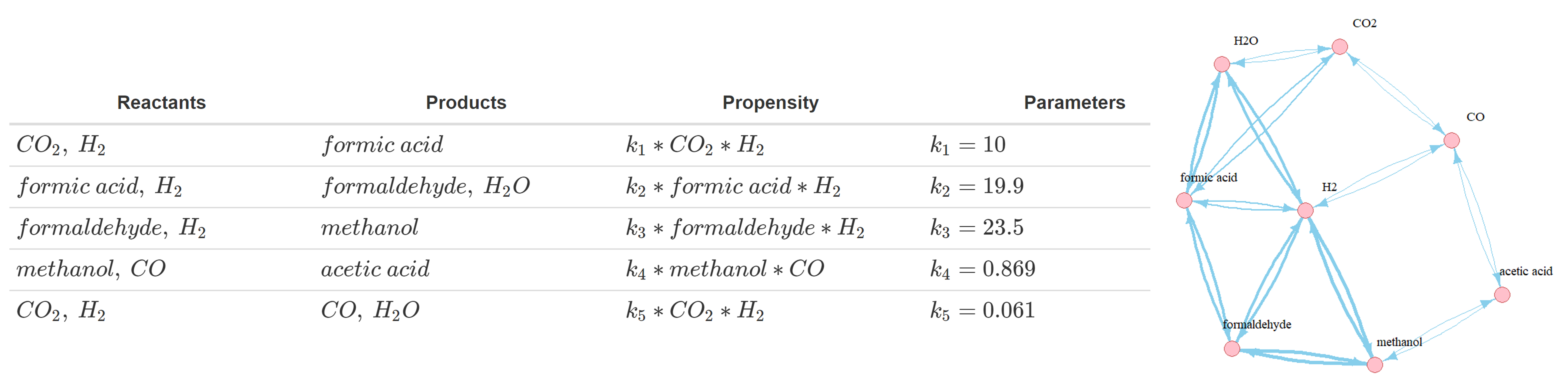
First, the propensity function: aj(x)dt = rate x Nreactants. It describes the probability that reaction j will occur in the next
infinitesimal time interval [t, t + dt], e.g. for the reaction A + B --> AB, the propensity is
kf x NA x NB, where kf refers to the rate of the reaction. See some examples of propensity functions
for the simulated network in the figure above. Second, the state-change vector, vj ≡ (v1j , . . . , vNj),
where v_ij is the change in the number of individuals in population i caused by one reaction of type j. For instance,
for A + B --> AB this will simply be [-1, -1, +1].
Sensitivity analysis
One of the questions that I was interested in was how the system behaved under different conditions. This is a slightly more unusually formulated question, as most modellers are usually interested in estimating single parameter values and combination. I was interested in a range of parameters under which a condition would hold e.g. under what kinetic conditions we could recover formaldehyde. Therefore, sensitivity analysis could reveal the relationships between the variables and their parameters. The literature and methods suited to answering broader and more abstract questions is still being developed for stochastic models. Moreover, many of the methods are suited to work with complete or partial data (i.e. fitting and optimisation for a set of parameters). In my report, I reviewed advanced brute-force (read, computationally expensive, for example Latin hypercube sampling) and heuristic (sacrificing exactness for performance; for example, simulated annealing and sequential probability ratio test (SPRT) or SParSE++) techniques for parameter estimation.
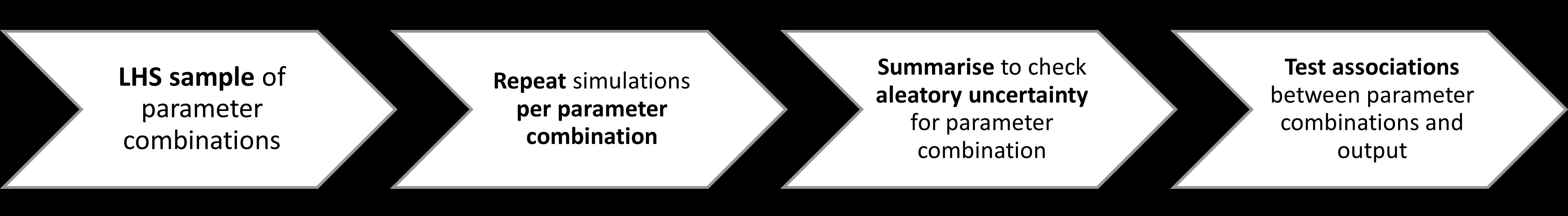
For simplicity's sake and as a proof of concept, I used a Latin hypercube sampling-based (LHS) sensitivity analysis technique,
using the pse R package. The steps are summarised below.
The partial rank correlation coefficients (PRCC) of every parameter against every molecule are given in Fig. 3. The ten kinetic parameters of the five CO2 fixation reactions were modelled as uniformly distributed with range [0.01,100]; N=50 Latin hypercube samples were drawn from the stratified parameter space. a. Partial rank correlation coefficients for every compound against every kinetic parameter; b. table with the reactions and their respective propensity functions (b in the subscript refers to “backwards reaction”); c. network visualisation which relates the reactants and products across CO2 fixation.
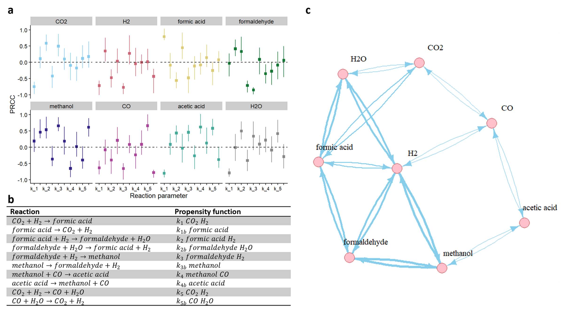
As expected, the individual chemical species were sensitive to the parameters which catalyse their reactions. Further, predictably,
in some cases the kinetics of the forward and backward reaction had opposite signs for their PRCCs. However, in other cases, the
impacts of upstream reactions was more prominent.
All chemical species were significantly sensitive to 4-5 parameters (n=37, in total). There were similar numbers
of significant positive and negative coefficients (n=18 and n=19, respectively). The quantity of a molecule was positively
correlated with the reactions which catalysed its formation and negatively with those catalysing its breakdown. This was especially
evident for limiting reactants or molecules which participated in multiple reactions, for example CO2, H2, H2O. Beyond this,
quantities were sometimes sensitive to the formation of their reactants, as seen, for example, for acetic acid. It would be
interesting to see how much further such trends extend in larger networks.
This analysis allowed the identification of bottlenecks in the network. In this case, the competition between CO and methanol was
highlighted qualitatively in the previous section. Sensitivity analysis revealed that methanol was
significantly positively correlated with several parameters for which CO was negatively correlated: k_2 (formaldehyde formation,
reactant for methanol formation), k_3 (methanol formation), k_5b (CO breakdown). Acetic acid, whose formation depends on both
methanol and CO supply, was also sensitive to these parameters.
This investigative project implemented a simple kinetic model of protometabolism. Whilst the network is incomplete,
it is growable and adaptable. The simulation output indicated that the model works accurately for reversible reactions.
More generally, reversible kinetic model has the potential of elucidating the dynamics of the network, but it could potentially
allow a realistic investigation of more scientifically interesting behaviours of metabolic flux to be captured. Further,
I adapted Latin hypercube sampling and sensitivity analysis to investigate the parameter space of the kinetic model.
While it would be premature to draw conclusions about the behaviour of the reversible CO2 fixation network, the PSE
results were coherent with the model simulation output.
Overall, although simple, the kinetic model proposed in this project could be applied to the investigation of stimulating
questions about the origin of metabolism, of the genetic code, of protocell proliferation, and about the origin of life.
The contribution of this work to the field lies beyond the kinetic model, extending into the discussion of the wider
challenges of parameter space exploration and validity of stochastic kinetic models. An important omission of
this work is the thermodynamic aspect of the metabolic network. As it is not negligible, the incorporation of
thermodynamic constraints in future models would be challenging but exciting.