Image processing for quantitative microscopy

Summer internship (2021) | Royal Microscopical Society

• GitHub

I spent the summer of 2021 with the Culley Lab at the Randall Centre for Cell & Molecular Biophysics (King's College London), funded by a Royal Microscopical Society summer studentship. I worked on a quantitative microscopy image processing project. My aim was to extract and quantify biologically relevant parameters from microscopy images of yeast microtubules, such as their number, length, curvature, etc..

Quantitative microscopy is an important field where methods are currently limited. Taking rigorous and reproducible measurements from microscopy data allows researchers to characterise novel phenomena or conduct statistical analysis on e.g. different conditions in a clinical trial. My summer project was a fun and stimulating challenge, as it involved comparing the performance of morphological operations on images to applied mathematics to deep learning approaches, and I gained valuable programming experience, using Python, ImageJ (macros), GitHub, and more.

How can image processing tools be used to quantify the linear structures present in fluorescence microscopy images of labelled tubulin in Schizosaccharomyces pombe (S. pombe)?

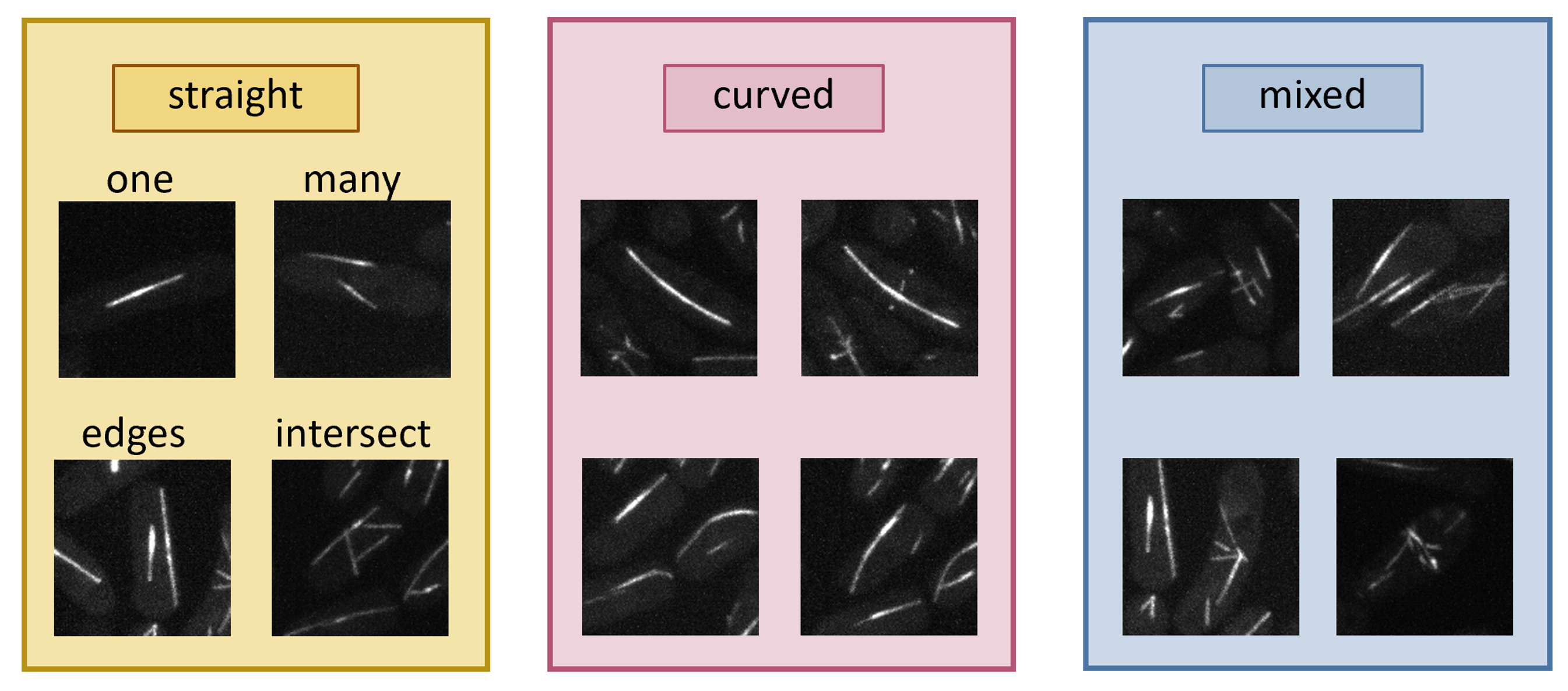
I wrote some ImageJ macros to easily curate data from the wider field confocal microscopy images of the microtubules. Several cases of lines can be identified readily. I chose to focus on parametrising straight lines first.

Thresholding and skeletonisation

First, I applied a global threshold to all images. This yielded binary images where, with a bit of post-processing, most of the labelled pixels belonged to lines.

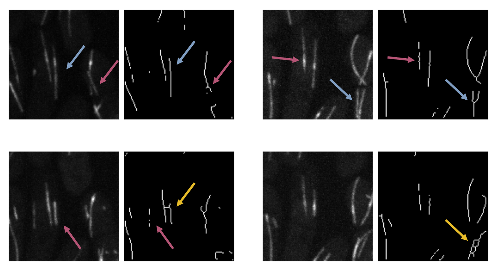
Then I "skeletonised" these images. Skeletonisation is a morphological operation, whereby in a group of adjacent pixels, outermost pixels are deleted until the object represented by the group of pixels is narrowed down to a single line. In theory, this is an efficient way to count the number of lines and measure their length/curvature. It is also great for creating a labelled training data set for a convolutional neural network.

I obtained some excellent results for single lines (straight and curved, shown with blue arrows). However, intersecting lines were dealt with more poorly. Although sometimes the results were comparable to the original case (pink arrows), some segmentations lead to severe artifacts (yellow arrows). The global threshold also broke up the lines, requiring more sophisticated algorithms.

The Linear Hough Transform

The Linear Hough Transform parametrises lines in terms of polar coordinates. So, instead of y = mx + c, the parametrisation in Cartesian coordinate space, we use the Hesse normal form, converting the gradient and intercept into y = [-cos(theta) / sin(theta)] x + [rho / sin(theta)]. Here, theta is the angle between the x and the norm, and rho is the length of the norm.

I am really brushing over the mathematics, but the advantage of this approach is that vertical lines can be parametrised too. In fact, I tried fitting lines using linear regression for the simplest of cases; however, the use-case of this method was more limited than the Hough transform.

A more intuitive way to think about the Hough transform is that every point in a plane can be thought of as infinitely many intersecting lines. Therefore, a point is converted to a line in Hough space, with unique rho and theta parameters. Therefore, For every point (x,y) and for every theta, calculate all values of rho using: rho = x cos(theta) + y sin(theta) (the Hesse normal).

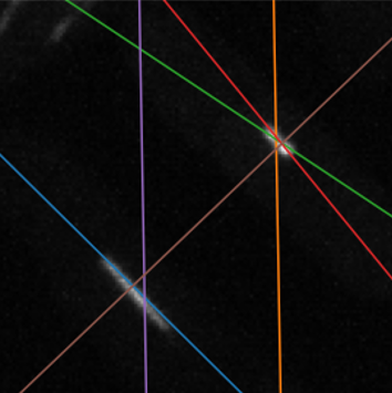
We can then use a peak-finding algorithm to detect peaks in polar Hough space. These peaks correspond to pairs, rho and theta, describing the lines in the image.

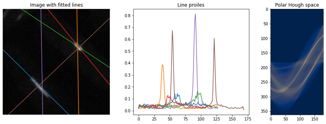
The plots below show the Hough transform and peak-finding algorithm from the sci-kit image Python library applied to an example of the skeletonised data (left) and another example of raw data (right). The accumulator in the Hough space is shown, with theta on the x-axis and rho on the y-axis.

It is notable that the Hough transform was sensitive to brighter lines and the hyperparameters of the peak-finding algorithm required manual fine-tuning. I tried to clean up the peaks, using their line profiles, by fitting Gaussian functions to the signal. This was effective in automatically discarding false positives if the number of peaks in the line profile was >1 or by thresholding the width of the signal.

Of course, these post-processing steps required extra coding and hyper-parameter tuning. However, I appreciated the challenge of pushing the Hough transform to its limit.

Extensions: deep learning

Although the methods I considered and hard-coded were effective for some use cases, I had only scratched the surface of what might appear to be a simple problem: labelling instances of lines in an image and quantifying simple parameters. To this end, deep learning for instance segmentation method that could cope with the full diversity of microtubule arrangements in a yeast cell. Although I did not have enough time to train my own Convolutional Neural Network (CNN), I had chosen an architecture, curated some data using ImageJ macros, begun labelling it manually and semi-automatically using skeletonisation, and even augmented my data to supply enough training data. I wanted to train a U-net from scratch and began setting up my Python environment with PyTorch and Keras.

The U-net is so called because of the U-shaped diagram of its architecture. It consists of an encoder branch, where the contracting path is composed of sequential down-sampling operations between convolutional layers. This reduces spatial information and increases feature information. The decoder branch holds the expansive path, where sequential transposed convolution and up-sampling operations propagate contextual information, helping the neural net localise features more accurately. This award-winning CNN has performed exceptionally with biomedical data.

Brilliant adaptations of the U-net exist, in which instead of performing pixel-to-pixel mapping (i.e. assigning image pixels to labels), the net is trained to perform pixel-to-shape mapping. StarDist and SplineDist are two excellent examples of this approach. Both of these tools have been used to segment nuclei in microscopy images. The final question, which remains unanswered for now, is whether this idea could be extended to mapping lines. However, as Sian, my supervisor, pointed out very detecting 1D objects in 2D data could be challenging for a CNN. Although I would have loved to conclude my summer project with such a standalone and robust tool, unfortunately, the summer flew by far too fast.

I deeply appreciated the opportunity to tackle a stimulating image processing problem in quantitative microscopy and thoroughly enjoyed pushing my solutions to their limit and looking for better alternatives. It was an invaluable research experience which taught me a lot about microscopy, Python, and image processing. Equipped with all these new image processing and segmentation skills in Python and ImageJ, I headed for my final year at UCL, where I joined the Simoncelli group at the London Centre for Nanotechnology and worked on segmenting the actin meshwork of activated T cells.